


Overview
In the modern data-centric world, the ability to efficiently manage dates and data points is crucial for a variety of analysis. The lubridate package in R has been designed to greatly simplify these date-related operations, thereby becoming an essential tool for survival analysis. A statistical method rooted in medical sciences, that has now been widely used in several areas as marketing analytics, thanks to its focus on analyzing the impact of time on different events.
When to use Survival Analysis
Survival analysis, also known as event-time analysis, is a valuable tool when dealing with particular types of data and analytical needs.
Applications of Survival Analysis
Survival analysis is a versatile tool applicable across various fields. For example, it helps compare treatment effectiveness in clinical trials, predict customer churning in marketing and estimate loan defaults in finance.
In general, this method is applicable for the following applications:
- Comparing Survival Rates: Compare survival times across different groups.
- Modeling Survival Data: Implementing the Cox Proportional Hazards model, to examine how various factors influence survival time.
- Predicting Future Events: Predicting when a future event, like a customer churn will occur.
Data Characteristics in Survival Analysis
In survival analysis, two types of data are crucial: - Time-to-Event Data: A variable indicating the time elapsed since the start to an event of interest, tracking the duration for each individual or unit in the study. - Survival Indicator: A binary (dummy) variable indicating whether the event of interest has occurred.
Your data also will consist of covariates. These are other variables that you believe might influence the time to event.
For measuring the time-to-event, we will use the R package lubridate. It simplifies the process of working with dates, allowing for easy calculation of time differences between events. Pairing the event-time variable with the survival indicator forms the foundation for survival analysis.
Censored Data
Survival analysis is particularly useful when your data includes censored observations, meaning not every subject or unit has experienced the event by the end of the observation period. It allows you to make informed predictions and comparisons despite incomplete data, which is a common challenge in longitudinal studies.
Censoring can occur in different ways: - Right Censoring: The most common form, where the event hasn't occurred by the end of the study, leaving the exact time of the event unknown. - Left Censoring: Occurs when the event's starting point is unknown, but its event is confirmed. - Interval Censoring: Happens when participants are not continuously observed, and the status of the event is only known at certain times.
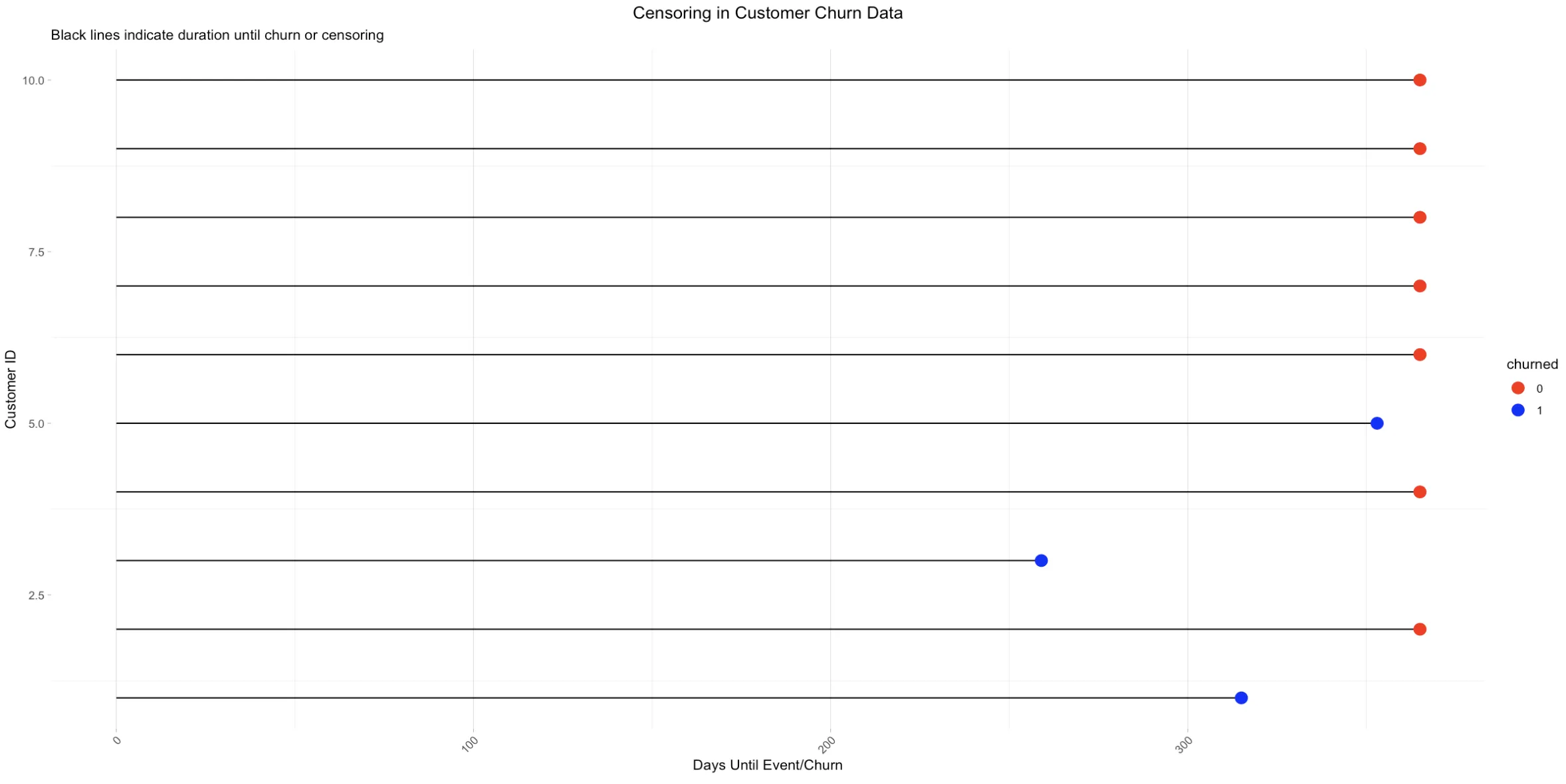
 Example
Here, subjects 1, 3, and 5 experience the event within the first year, while subjects 2, 4, 6, 7, 8, 9, and 10 do not. These latter subjects are 'censored' after one year, meaning we only know they didn't encounter the event in the first year, but their status thereafter is unknown.
Lubridate
This section will guide you through the basic functionalities of lubridate, helping you manage and manipulate date-time data more efficiently.
Starting with lubridate
In this section, we introduce the basics of the lubridate package in R, focusing on installing the package, parsing dates and times, handling time zones, manipulating dates, and performing various operations.


# Download the code in the top right corner
Advanced lubridate functions
Here, we explore more advanced features of lubridate, including custom parsing techniques, advanced arithmetic, time zone manipulations, and integration with other R packages for enhanced data analysis.
# Download the code in the top right corner
Calculating Survival Times Using Lubridate
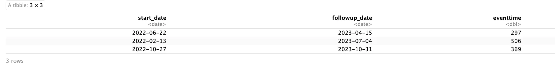
In survival analysis, data often includes two date columns, like start_date and followup_date. R may initially treat these as character strings, requiring conversion into date objects. The ymd() function in the lubridate package is useful for converting strings in the "year-month-day" format into dates.
To calculate the event-time or the survival-time variable, the interval between the two dates is measured. The %--% operator in lubridate creates an interval object, which can then be converted into a duration in seconds using as.duration(). The difference in days is obtained by dividing this duration by ddays().
# Load necessary packages
## install.packages(c("tibble","dplyr","lubridate"))
library(tibble)
library(dplyr)
library(lubridate)

# Example dataset with start and follow-up dates
date_ex <- tibble(
  start_date = c("2022-06-22", "2022-02-13", "2022-10-27"),
  followup_date = c("2023-04-15", "2023-07-04", "2023-10-31")
  )

# Convert character columns to date columns
date_ex$start_date <- ymd(date_ex$start_date)
date_ex$followup_date <- ymd(date_ex$followup_date)

# Create an event-time variable
date_ex <- date_ex %>%
  mutate(
    eventtime = as.duration(start_date %--% followup_date) / ddays()
    )

# Display the updated data frame
print(date_ex)
Now you have properly calculated the durations, with dates formatted and intervals measured in the unit of choice, you now can dive into survival Analysis!
Survival Analysis
With our date data now prepared and structured, we can begin examining the factors that influence whether a certain event occurs or not in survival analysis. This investigation starts with the concept of the Survival Function, a fundamental aspect of survival analysis.
The Survival Function
The Survival Function, typically denoted as
$S(t)= P(T>t) =1−F(t)$
- S(t): This is the survival function at time t. It represents the probability that the subject or unit of study survives longer than time t.
- P(T>t): This term denotes the probability that the time until the event occurs (denoted by T) is greater than a specific time point t. Essentially, it's the likelihood that the event of interest has not occurred by time t.
- 1−F(t): F(t) is the cumulative distribution function (CDF) of the time until the event. It gives the probability that the event has occurred by time t. Thus, 1−F(t) is the probability that the event has not occurred by time t.
The Kaplan-Meier Estimator
In practical terms, to get an understanding of the survival function or survival probability, the Kaplan-Meier estimator is commonly used to estimate S(t). Furthermore, the Kaplan-Meier curve gives a visual representation of the survival probability over time, offering insights into the overall survival probability.
For our analysis, consider a scenario where you're managing a subscription service and aiming to understand customer churn. You record when customers unsubscribe, but not all will have unsubscribed by your analysis time, leading to right-censored data.
The Kaplan-Meier Estimator in R
To conduct a Kaplan-Meier estimation in R, follow these steps:
- Dataset Preparation: Ensure your dataset includes event times and indicators for event occurrence or data censoring.
- Creating the Survival Object: Use the
Surv()function from thesurvivalpackage to create a survival object. This object combines time-to-event data and the event indicator, allowing survival analysis methods to accurately account for event timing and event occurrence or censoring. - Calculating the Kaplan-Meier Estimate: Use the
survfit()function to compute the Kaplan-Meier estimate. This function estimates the survival function, either for the overall data or segmented into groups.- Basic syntax: survfit(Surv(time, event) ~ 1, data = your_data).
1. ~ 1 calculates the overall survival curve without data grouping.
2. For group comparisons, replace 1 with a grouping variable.
3. The output of
survfit()includes estimated survival probabilities at different time points, the number of subjects at risk, and the number of events. - Between group significance test: Log-rank test.
1. Use the
survdiffformula to obtain the p-values 2. Compares survival times, weighting all observations equally.
- Basic syntax: survfit(Surv(time, event) ~ 1, data = your_data).
1. ~ 1 calculates the overall survival curve without data grouping.
2. For group comparisons, replace 1 with a grouping variable.
3. The output of
- Visualizing the Estimate: Use the
ggsurvplot()function for Kaplan-Meier estimate visualizations. It combines ggplot2 aesthetics with a risk table, displaying subjects at risk over time.
# Load the survival package
library(survival)

# 1. Dataset Preparation
## Convert to Date objects
data$start_date <- ymd(data$start_date)
data$event_date <- ymd(data$event_date)

## Calculate time to event or censoring
data$time_to_event <- interval(start = data$start_date, end = data$event_date) / ddays(1)

## Create the censoring indicator (1 if event occurred, 0 if censored)
data$censoring_indicator <- ifelse(is.na(data$event_date), 0, 1)

## 2. Creating the Survival Object
surv_obj <- with("YOUR DATASET",
                Surv(time = "EVENTTIME VARIABLE", # Eventtime Variable
                     event = "CHURNING / CENSORED VARIABLE")) # Churning / Censored Variable

# 3. Compute the Kaplan-Meier estimate
km_fit <- survfit(surv_obj ~ "COVARIATE 1" + "COVARIATE 2" + ... , data = "DATASET")
 ## km_fit <- survfit(surv_obj ~ 1) implies a model without covariates.

## Test for significance between groups
survdiff(surv_obj ~ "GROUPING VARIABLE", data = "DATASET")

# 4. Visualizing the Estimate
## Plot the Kaplan-Meier curve
km_plot <- ggsurvplot(
  km_fit, # Kaplan-Meier estimate
  conf.int = FALSE, # Omit Confidence Interval
  risk.table = TRUE, # Provide a Risk Tabe
  surv.median.line = "hv", # Add a median horziontal line
)

## Display the plot
km_plot
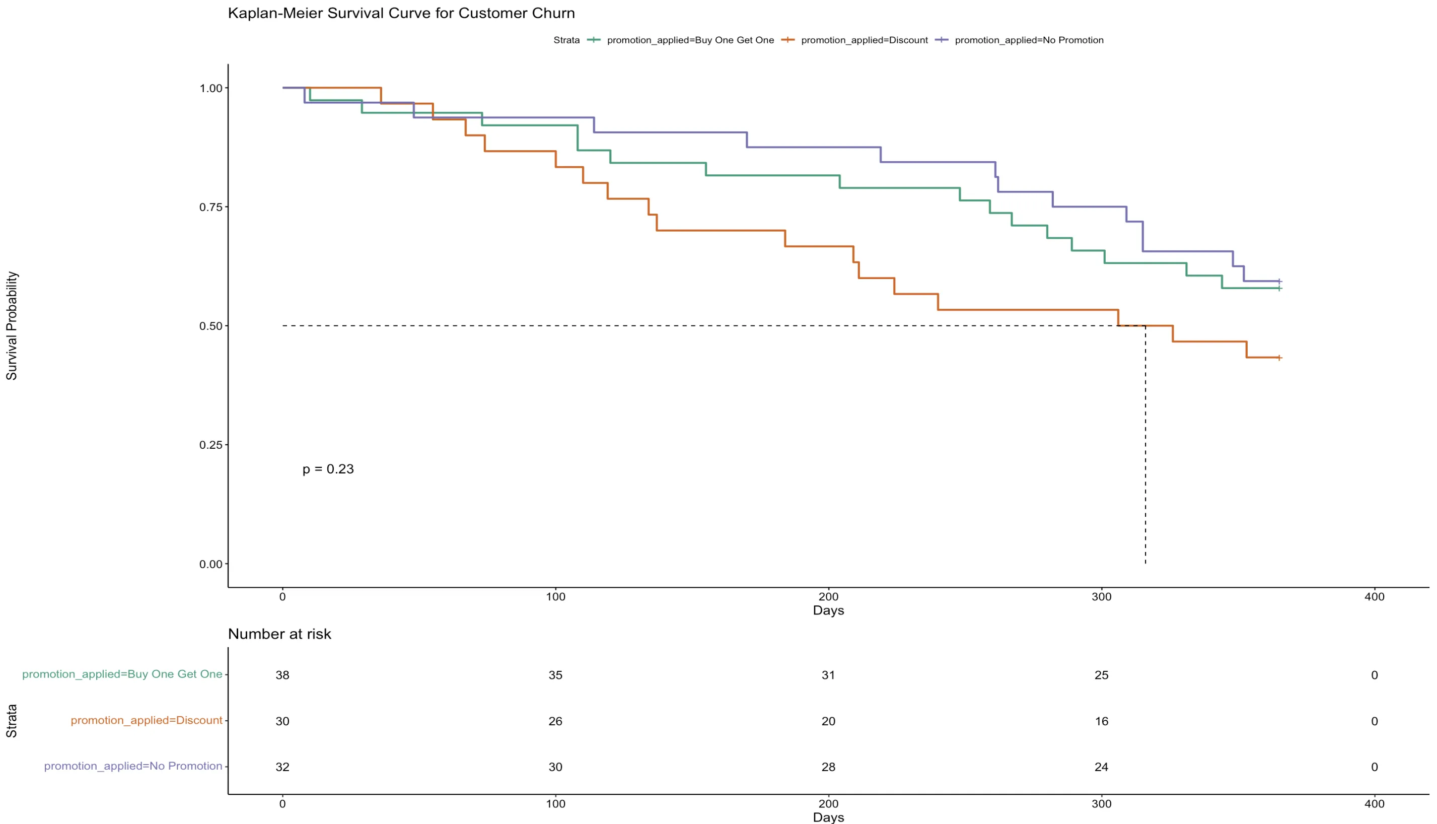
This Kaplan-Meier curve illustrates customer churning across three promotional strategies over time. The y-axis quantifies the likelihood of customers staying, while the timeline is plotted along the x-axis. Each promotional group—Buy One Get One, Discount, and No Promotion—shows similar retention patterns, as the curves proceed with only slight differences.
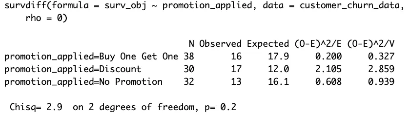
The survdiff function's output, with a p-value of 0.2, indicates no statistically significant differences in retention across these promotional strategies. The lack of significant drop-offs suggests that the promotions have a marginal impact on churn rates. This insight suggests promotions, in this case, does not significantly influence customer loyalty.
The Cox Proportional Hazard Model
The Cox Proportional Hazards model is a key tool in survival analysis for understanding how different factors, known as covariates, affect the time until an event occurs. This model allows you to look at several factors at once and see how each one independently influences survival time, even when other factors are considered. It's a powerful tool for identifying significant factors and quantifying their influence on the probability and timing of the event occurring.
The model's formula is expressed as:
$h(t|X_{i}) = h_{0}(t)exp(β_{1}X_{i,1}+...+β_{p}X{i,p})$
The formula combines a starting risk level with the influence of specific factors and their strengths to calculate the chance of an event happening at any particular time.
The Cox Proportional Hazard Model in R
To apply the Cox model in R, the coxph() function from is used. This function requires again the Surv() object, and a formula specifying the model's covariates.
Results can be summarized using the tbl_regression() function from the gtsummary package, with parameters set to show the hazard ratio (HR) instead of the logarithm of the hazard ratio.
The HR compares the hazard rates between groups, with a value greater than 1 indicating an increased event rate and a value less than 1 indicating a reduction. Note that the HR states the rate of occurrence, not the probability of occurrence.
 Tip
TipEnhanced Presentation
For a more effective presentation of the results, consider using the ggforest() function to generate a forest plot. This plot graphically displays the HRs for all variables in the model, along with their confidence intervals, providing a visual and comprehensive summary of the findings.
The codeblock underneath contains a template for estimating the Cox Proportional Hazard Model in R:
# Load necessary packages
library(survival)
library(gtsummary)
library(ggplot2)

# Fit a Cox proportional hazards model
fit.coxph <- coxph(Surv(time = "Eventtime_Variable",
                        event = "Churning_Censored_Variable") ~ "Covariate_1" + "Covariate_2",
                        data = "Your_dataset")

# Create a summary table with Hazard Ratios
tbl <- tbl_regression(fit.coxph, exp = TRUE)

# Visualize the results with a forest plot
ggforest("fit.coxph", data = "Your_dataset")

# Print the forest plot
print(forest_plot)
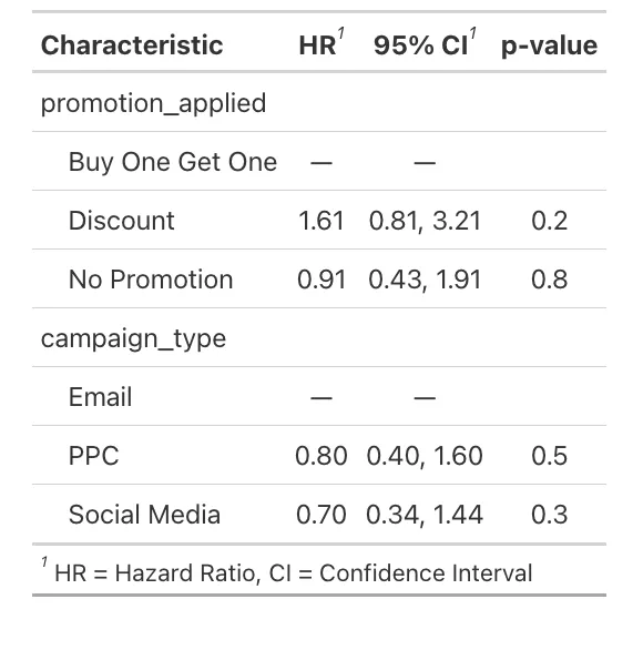
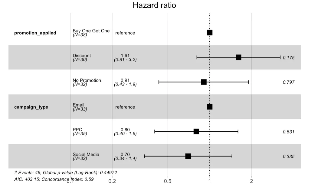
The forest plot visualizes the Hazard Ratios (HRs) for different categories of promotion and campaign types. The reference category for promotion_applied is "Buy One Get One," and for campaign_type, it's "Email." - The "Discount" promotion has a HR of 1.61, suggesting a 61% increase in the hazard compared to the "Buy One Get One," but this is not statistically significant (p-value 0.175). - The "No Promotion" category has a HR close to 1 (0.91), indicating no substantial change in hazard compared to the reference. - For campaign_type, "PPC" (Pay-Per-Click) and "Social Media" have HRs below 1 (0.80 and 0.70, respectively), suggesting a lower hazard of the event occurring compared to "Email," but again, these are not significant.
 Summary
This building block contains an extensive overview of survival analysis and its application in various fields, emphasizing the role of the lubridate package in R for effective date management.
Key takeaways include:
- Importance of Date Management: Demonstrating how lubridate simplifies handling dates and times in R, crucial for survival analysis.
- Survival Analysis Explained: Introducing survival analysis, its significance in assessing the timing of events, and its applicability from product lifecycles to customer churn prediction.
- Practical Application: Providing practical examples, including visualizations like the Kaplan-Meier curve and the Cox proportional hazards model, to illustrate survival probabilities and the effectiveness of various strategies in scenarios like customer retention.
Source Code
Here is the source code for the analysis:
# Download the file in the top right corner